DART: Decoded Attention over Recurrent States

DART illustration: a dart hits a target among sequence tokens, representing selective retrieval.

Modern large language models

Modern language models largely build on three families: Transformers, recurrent models, and hybrids.

Transformers represent history as token-level keys and values. At each step, a query compares against earlier keys and retrieves a weighted combination of their values. This gives the model explicit, content-dependent access to previous positions. The cost grows with context: full attention requires quadratic training compute, and autoregressive inference maintains a KV cache whose size grows linearly with sequence length.

Recurrent models, including state space models (SSMs) and linear attention, compress history into a compact state that is updated as new tokens arrive. Mamba and Mamba-2 use input-dependent state dynamics to control what is written, retained, and read. Linear attention also admits a recurrent formulation, accumulating key–value associations in a state. These formulations enable linear-time sequence processing and a fixed-size recurrent memory during inference. Compression, however, can make precise retrieval difficult, especially when the query is unknown at the time information is written. Zoology studies this recall gap between attention and efficient recurrent alternatives.

Hybrid models combine recurrent efficiency with attention-based retrieval. Architectures such as Jamba and Zamba interleave recurrent computation with attention layers, improving the balance between efficiency and model quality. These designs still maintain two forms of memory: token-level KV caches for attention and compact states for recurrence.

This motivates the central question of DART:

Can a unified memory representation support both recurrent compression and attention-style retrieval?

A unified memory representation

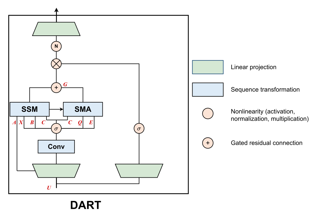
Mamba-2 provides a natural starting point through state space duality (SSD). SSD shows that a selective state space layer can also be written as structured causal attention: its coefficients \(A,B,C,X\) correspond to the attention roles of decay, keys, queries, and values. This connects recurrent computation and attention through the same underlying state representation.

The recurrent update and readout take the form

\[H_t = a_t H_{t-1} + B_t^\top X_t, \quad Y_t^{\mathrm{SSM}} = C_tH_t.\]

The state \(H_t\in\mathbb{R}^{N\times P}\) can therefore be viewed as a compressed KV cache. The outer product \(B_t^\top X_t\) writes a token-dependent association into it, while \(a_t\) controls how the previous state carries forward. The readout \(C_tH_t\) uses the current token’s read vector to extract a value from this accumulated memory.

The key observation behind DART is that Mamba-2 reads values from the compressed KV cache, but does not decode keys from that cache for attention. Decoding keys as well would make it possible to compare a query against compressed recurrent memories and retrieve the relevant information from them.

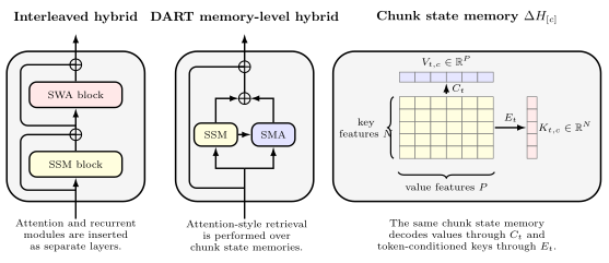
Interleaved recurrent and attention layers compared with DART, followed by a matrix showing value and key readouts from a shared chunk state. — **Figure 1.** Two ways to combine recurrence and attention, and the matrix representation used by DART. SWA denotes sliding-window attention in the illustrative interleaved hybrid. The right panel previews the two directions in which a chunk state can be read.

SSD also provides an efficient chunkwise algorithm. Alongside the recurrent outputs, it computes each chunk’s contribution to the state. DART retains these contributions as chunk state memories. Each stored matrix represents what a particular chunk writes, giving retrieval access to individual compressed portions of the history.

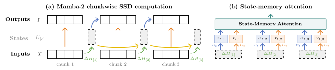
Chunkwise Mamba-2 computation produces outputs and local state contributions; the retrieval branch reads historical contributions through E and C to construct keys and values. — **Figure 2.** Constructing and retrieving chunk memories. The left panel distinguishes local contributions from cumulative boundary states. The right panel illustrates retrieval after the three displayed chunks have become historical.

This leads to state-memory attention (SMA). For the current token, \(C_t\) decodes a value and \(E_t\) decodes a key from each completed historical chunk memory. The query \(Q_t\) scores those keys, and attention combines the corresponding values. DART adds the retrieved readout to the native Mamba-2 output through a gated residual connection.

The two branches share the chunk state memories: recurrence compresses tokens into states, and attention retrieves from those states. The following sections explain how these memories are formed and how their keys and values are decoded.

From chunk contributions to stored memories

Mamba-2’s chunkwise computation divides a sequence into chunks of \(S\) tokens. Alongside local outputs, it computes each chunk’s contribution to the recurrent state. For chunk \(c\), ending at position \(e(c)\), that contribution is

\[\Delta H_{[c]} = \sum_{s\in[c]} \left(\prod_{k=s+1}^{e(c)} a_k\right) B_s^\top X_s.\]

Each matrix \(\Delta H_{[c]}\in\mathbb{R}^{N\times P}\) summarizes the associations written within that chunk.

DART retains the individual contribution matrices as chunk state memories. The native recurrent state continues to evolve, while SMA gains access to a sequence of compressed historical memories.

Decoding keys and values for the current token

For a token at position \(t\), the block input \(U_t\) produces three vectors:

\[Q_t = U_t W_Q, \quad C_t = U_t W_C, \quad E_t = (U_t W_E)^\top.\]

The query \(Q_t\in\mathbb{R}^{1\times N}\) determines which chunk memories receive attention. The native Mamba-2 read vector \(C_t\in\mathbb{R}^{1\times N}\) extracts values. The verifier \(E_t\in\mathbb{R}^{P\times 1}\) reads the value axis to construct a key for each memory.

For a historical chunk \(c\), the two decoded representations are

\[V_{t,c} = C_t\Delta H_{[c]} \in\mathbb{R}^{1\times P}, \quad K_{t,c} = \Delta H_{[c]}E_t \in\mathbb{R}^{N\times 1}.\]

The stored object is a matrix; its decoded key and value depend on the current token. The same chunk memory can yield different representations at different positions. Both readouts are token-conditioned through \(C_t\) and \(E_t\), with a separate query \(Q_t\) used to score the decoded key.

The attention calculation then has a familiar form:

\[\ell_{t,c} = \frac{Q_t K_{t,c}}{\sqrt{N}}, \quad g_{t,c} = \operatorname{softmax}_{c<c(t)}(\ell_{t,c}), \quad R_t = \sum_{c<c(t)} g_{t,c}V_{t,c}.\]

Here \(c(t)=\lceil t/S\rceil\) is the current chunk. For clarity, these equations omit normalization in the score computation. The implementation applies RMS normalization to \(Q_t\) and \(E_t\), and scales the state rows by their inverse root mean square when decoding keys.

The retrieved value enters as a gated correction to the native state readout:

\[G_t = \operatorname{SiLU}(U_t W_G), \quad Y_t = C_tH_t + G_tR_t.\]

The gate \(G_t\) is scalar, and \(W_G\) is initialized to zero. The retrieval contribution therefore starts at zero and is learned during training. The surrounding Mamba-2 block processes the combined readout through its usual output operations.

Figure 3. The complete DART block, reproduced from the paper's PDF figure. The SSM branch supplies chunk memories to SMA, and both branches use the read vector C. The gate G controls the retrieved correction.

Making retrieval efficient

DART reuses Mamba-2’s chunkwise computation to construct the memories shown in Figure 2. Efficient retrieval requires an additional step: a custom FlashAttention-style kernel for SMA.

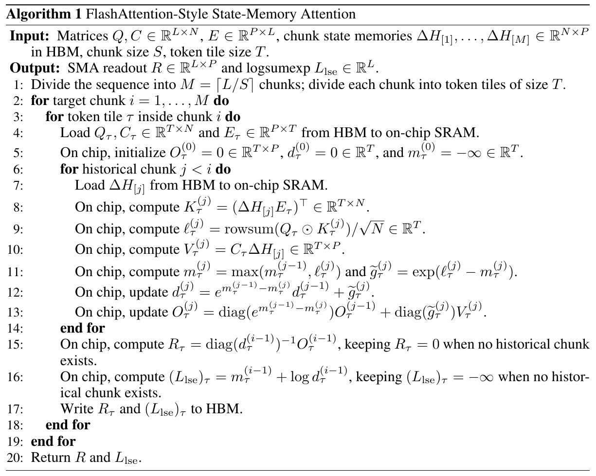
The kernel processes a tile of queries while streaming through historical chunk matrices. It decodes their keys and values in on-chip memory, updates an online softmax, and accumulates the retrieved output. Decoded keys, values, logits, and attention weights remain temporary quantities. The forward pass writes the readout and log-sum-exp statistics to device memory; backward computation reconstructs the temporary quantities as needed.

This avoids materializing large token-by-chunk intermediate tensors. It reduces memory traffic while retaining the additional arithmetic required by SMA.

Algorithm 1 from the DART paper: tiled SMA forward computation, decoding historical-state keys and values on chip and accumulating an online softmax. — **Algorithm 1.** FlashAttention-style SMA, reproduced from the paper. Each query tile visits only earlier chunks. Keys, values, logits, and softmax weights are computed on chip; only the readout and log-sum-exp statistics are written to HBM.

Cache size

Let the sequence length be \(L\) and the number of chunks be \(M=\lceil L/S\rceil\). A matched token-level attention head with key and value dimension \(P\) stores approximately \(2LP\) elements. DART’s historical chunk matrices require approximately \(MNP\) elements. Their leading, length-dependent cache ratio is

\[\frac{MNP}{2LP} \approx \frac{N}{2S}.\]

At \(N=128\) and \(S=256\), the ratio is \(1/4\): 75% less length-dependent cache under this matched comparison. For example, at \(L=4096\) and \(P=64\), the chunk matrices contain 131,072 elements per head, compared with 524,288 elements for token keys and values.

This comparison assumes the same element precision and excludes fixed recurrent state, small normalization statistics, model weights, and other runtime allocations. It describes the dominant historical cache term. Total device-memory savings depend on the complete implementation and the attention baseline’s head-sharing configuration.

Compute cost

Each token can visit roughly \(L/S\) historical chunks, with key and value decoding costing \(O(NP)\) per visit. The added SMA computation is

\[O(LMNP)=O\!\left(\frac{L^2NP}{S}\right).\]

For fixed \(N\) and \(S\), this is quadratic in sequence length, on top of Mamba-2’s linear-time state computation. Relative to token-level attention’s \(O(L^2P)\) arithmetic, the leading ratio is \(N/S\). Actual latency also depends on kernel utilization and memory movement; this ratio alone gives no wall-clock speedup guarantee.

Smaller chunks preserve more separately addressable memories and increase retrieval work. Larger chunks reduce cache and computation while compressing more information into each memory. Chunk size controls this trade-off.

Experiments

Associative recall

Multi-query associative recall, or MQAR, asks a model to remember several key–value pairs and predict the associated value when a key reappears. The paper compares DART and Mamba-2 at matched model widths and state sizes, alongside a Transformer++ baseline.

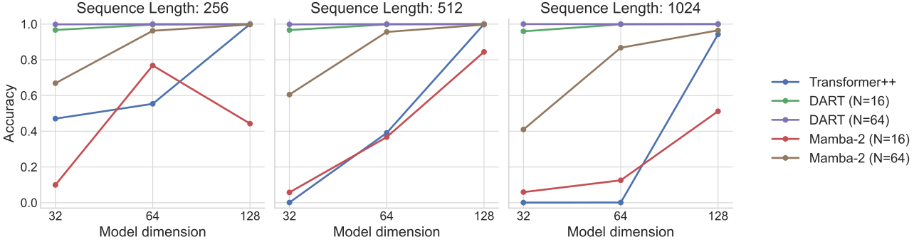
MQAR accuracy at sequence lengths 256, 512, and 1024, showing DART outperforming matched Mamba-2 variants across model widths 32, 64, and 128. — **Figure 4.** MQAR results from the paper. Each panel fixes sequence length and varies model width; N denotes state size. These experiments use a chunk size of 16. Accuracy is plotted on a zero-to-one scale.

At \(N=64\), DART reaches near-perfect recall across all tested widths and sequence lengths. Even with \(N=16\), it exceeds Mamba-2 with \(N=64\) at matched widths in these experiments. The gains suggest that selective access to stored states can make compressed associations more useful.

The chunk size here is \(S=16\). The separate 75% cache-saving example uses \(S=256\) and \(N=128\); that percentage should not be assigned to this MQAR setting.

Language modeling and extraction

The language models are pretrained on the Pile for 100 billion tokens. DART adds fewer than 3% parameters to the corresponding Mamba-2 backbones. The main language-modeling configuration uses \(S=256\) and \(N=128\).

Table 1. Pretraining on the Pile. Complete table reproduced from the DART paper. — **Table 1. Pretraining on the Pile.** Validation metrics after 100 billion training tokens. Accuracy is a percentage; lower perplexity and higher accuracy are better.

Table 2. Zero-shot downstream evaluation. Complete table reproduced from the DART paper. — **Table 2. Zero-shot downstream evaluation.** All accuracy entries are percentages. LAMBADA PPL is perplexity; accₙ denotes length-normalized accuracy. Avg. averages the seven accuracy metrics. DART rows with chunk sizes 64 and 32 evaluate the same checkpoints trained with a chunk size of 256.

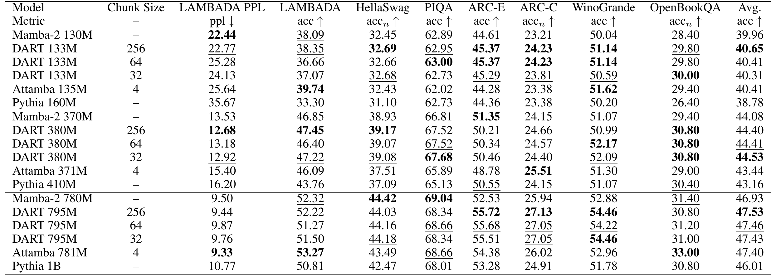
The average covers seven downstream accuracy metrics reported in the paper. General language-modeling quality stays close to the backbone, with modest average downstream gains. Most examples in these downstream benchmarks are shorter than 256 tokens, so many do not activate historical-chunk retrieval at this chunk size. This evaluation primarily checks that training with SMA preserves the recurrent branch’s general capability.

The changes are larger on information extraction. SWDE asks for attribute values from web pages; FDA asks for values associated with requested keys in regulatory documents. Both are scored with contains accuracy, which checks whether the generated response contains the expected answer.

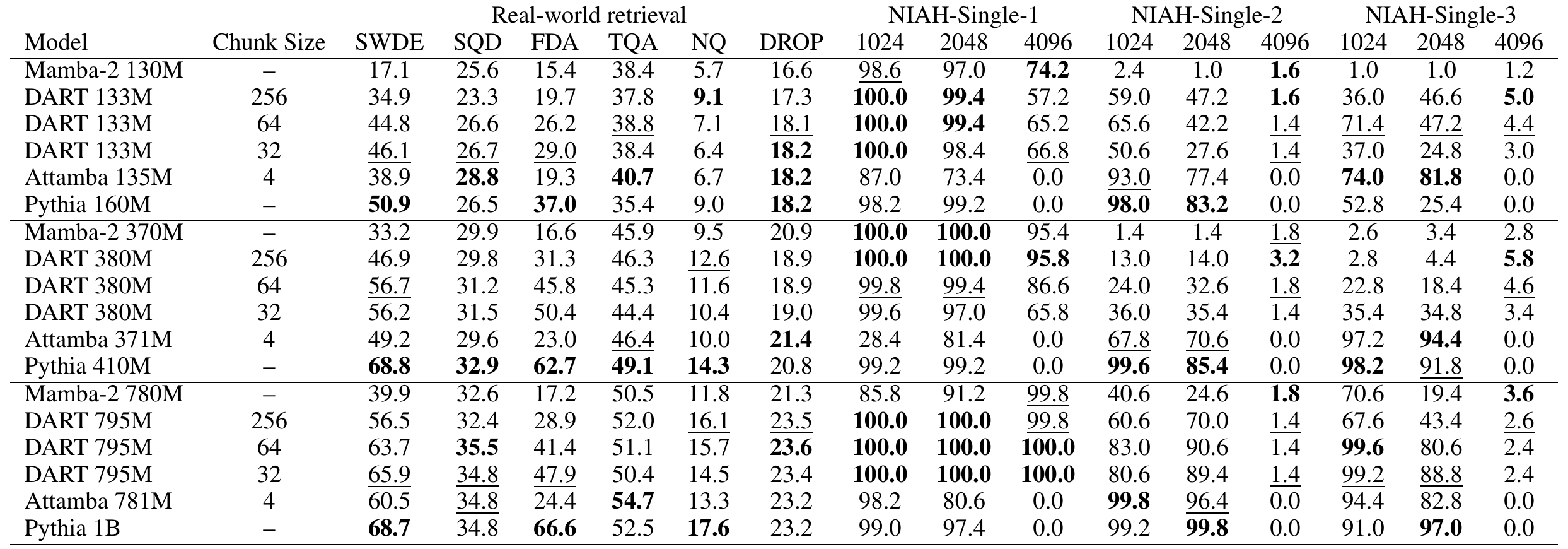
Table 3. Real-world and synthetic retrieval. Complete table reproduced from the DART paper. — **Table 3. Real-world and synthetic retrieval.** All entries are percentages; higher is better. Real-world tasks use contains accuracy. SQD denotes SQuAD Completion, TQA denotes TriviaQA, and NQ denotes Natural Questions. NIAH uses 500 examples at each context length; column labels give context lengths in tokens. All model baselines and evaluation chunk sizes are included.

These entries use DART’s main \(S=256\) setting. Synthetic needle-in-a-haystack tests also show substantial gains in several configurations: for example, on NIAH-Single-2 at 2,048 tokens, the 780M/795M comparison improves from 24.6% to 70.0%.

The results vary by task and context length. Many 4,096-token NIAH-Single-2 and Single-3 settings remain difficult. There are regressions as well: on NIAH-Single-1 at 4,096 tokens, DART 133M scores 57.2% versus Mamba-2 130M’s 74.2%. Full-attention Pythia remains stronger on several extraction and question-answering metrics, and Attamba is strong on several synthetic retrieval settings. The complete comparisons above show both the retrieval gains and the settings where other architectures remain stronger.

What the ablations reveal

Removing the SMA branch at evaluation time tests how much the trained model relies on retrieval from historical chunk states. It strongly reduces extraction accuracy and MQAR recall. The NIAH effects depend on the task and context length, so the SMA branch should not be read as a uniform improvement on every retrieval metric. This intervention uses a trained DART checkpoint; it is distinct from training a standalone Mamba-2 baseline.

Table 4. Removing the SMA branch: retrieval. Complete table reproduced from the DART paper. — **Table 4. Removing the SMA branch: retrieval.** All entries are accuracies in percent, with chunk size 256. Rows marked w/o SMA use the same trained DART checkpoint with its SMA residual readout removed during evaluation.

Table 5. Removing the SMA branch: MQAR. Complete table reproduced from the DART paper. — **Table 5. Removing the SMA branch: MQAR.** Test accuracy in percent, with state size 16 and chunk size 16. L is the sequence length. Each pair compares a trained DART model with and without its SMA branch during evaluation.

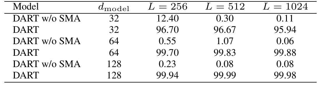
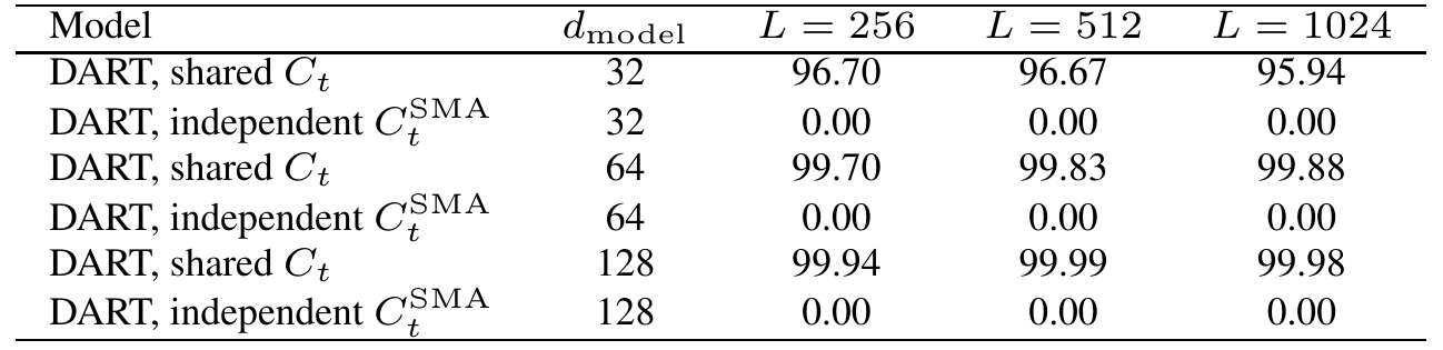
Sharing the native SSM read vector \(C_t\) also matters. In the memory-constrained MQAR setting below, the shared design achieves high recall, while the otherwise matched variants with an independent SMA read vector remain at zero accuracy. This result supports sharing \(C_t\) for decoding historical memories in this tested setting.

Table 6. Sharing the SSM read vector: MQAR. Complete table reproduced from the DART paper. — **Table 6. Sharing the SSM read vector: MQAR.** Test accuracy in percent, with state size 16 and chunk size 16. These are separately trained, otherwise matched variants with a shared or independently parameterized value-side read vector.